5.2. Procedural Generation
Procedular generation is just writing code to define vertices and polygons, instead of loading them or creating them manually.
We have to remember to:
- Define points (vertices);
- Define how to draw them (elements + primitives); and
- Define normals.
- (optionally) add texture coordinates and textures.
Random numbers are very useful for procedural generation, but remember that computers cannot really generate random numbers.
Instead, they generate pseudo-random numbers by using a formula and an initial seed.
If you provide the same seed to a random generator, you will always come up with the same “random” numbers.
5.2.1. Self-similar objects
If a portion of the object is looked at more closely, it looks exactly like the original object.
For example, a snowflake or a rocky mountain.
5.2.1.1. L-systems
An L-system is a simple way to represent self-similar objects:
- The \(F\) means move one unit forward.
- The \(+\) means turn clockwise.
- The \(-\) means turn counter-clockwise.
- The \([\) means start a new branch.
- The \(]\) means end a branch.
So L-systems work by iterations. Each iteration replaces an \(F\) with the complete L-system definition.
So the first iteration would look like this:
And the second iteration would look like this:

5.2.2. Skylines and landscapes
5.2.2.1. Heightfield or DEM
A heightfield is just an array of arrays of height (Y) values.
It can look something like this:
[
  [5.6, 3.4, 3.7, 3.5, 4.8],  # z == 0
  [3.5, 3.9, 4.9, 7.9, 7.5],  # z == 1
  [2.3, 3.0, 4.0, 3.7, 3.2],  # z == 2
  [3.5, 3.9, 4.9, 7.9, 7.5],  # z == 3
  [3.2, 3.9, 5.3, 4.7, 8.1],  # z == 4
]
For each of the elements of the array, x is increasing (from 0 to 4).
Eventually, we end up with a terrain, that may look something like this:

Then we can draw the triangles. And calculate the normals.
In order to achieve a more random-looking terrain, there are a few functions we can use.
5.2.2.1.1. Random mid-point displacement
Set values for the first and last elements of the heightmap, and then the middle element will be randomised between the two beside it.
So on the first iteration, there would be 3 elements.
On the second iteration, there would be 5 elements, then 7, and so on.
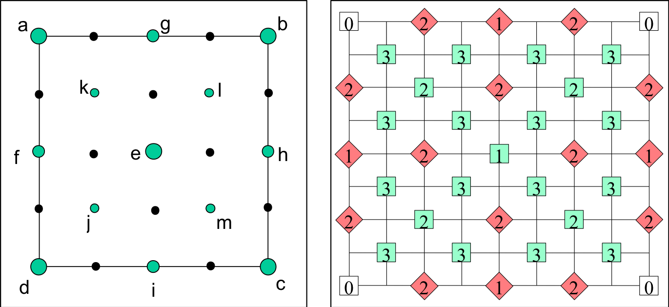
The order in which elements on a 3D height-map would be calculated would be as follows:
5.2.2.1.2. Noise functions
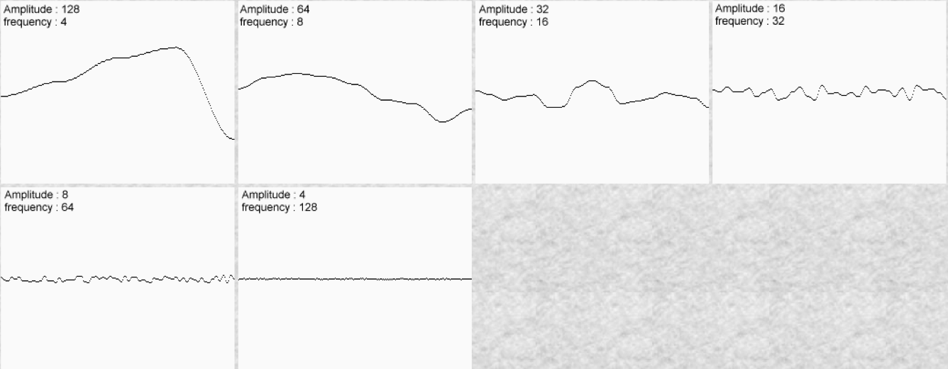
Perlin noise is generated by adding multiple noise functions together, at increasing frequency and decreasing amplitude:
A “better” noise function is Simplex noise.
Poisson faulting adds detail to a sphere by making it grow at random positions, like so:
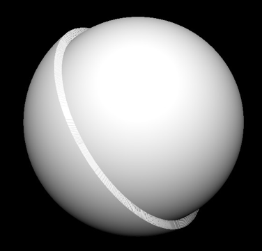
Doing that many times (without making the growing too large) will result in added detail for e.g. asteroids or planets.
However, Poisson faulting is slow at \(O(N^3)\).